WTSFest Philly is back on October 1st!
WTSFest Philly is back on October 1st!

Author: Jess Peck
Last updated: 29/05/2024
Consistently, one of the most difficult parts of SEO seems to be proof. It can be hard to prove your changes did anything: never mind making predictions about the future. Sometimes we over-rely on “it depends” and “Google Algo Updates” to hide these difficulties with forecasting.
SEO professionals often grapple with the uncertainty of their strategies' outcomes and the ever-changing algorithms of search engines. This uncertainty makes it challenging to confidently attribute changes in website traffic or rankings to specific SEO actions.
This is where math, statistics, and advanced analytical tools come into play. In this article, we will look at three tools – ARIMA (AutoRegressive Integrated Moving Average), Facebook's Prophet, and Causal Impact - and demonstrate how they can be leveraged to analyze SEO data effectively.
First, a brief overview of the tools:
ARIMA: A classic in time series forecasting, ARIMA models are excellent for understanding and predicting future data points in a series. For SEO purposes, ARIMA can be used to forecast website traffic trends and assess the effectiveness of SEO strategies over time.
Facebook's Prophet: This is useful for predicting future trends based on historical data. It can be particularly helpful for anticipating the effects of seasonal changes, marketing campaigns, or other events.
Causal Impact: Developed by Google, this tool is designed to estimate the causal effect of an intervention on a time series. For SEO, it can help in understanding the impact of specific changes or updates on website traffic or rankings.
If you just want to get to the code, you can use the colab and skip the explanation. For the rest of us, let's dive in.
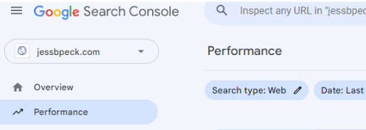
Google Search Console (GSC) provides valuable insights into how your site performs in Google Search.
GSC data can be sampled, especially for larger sites or longer date ranges. This means not every single query or click is recorded. There's also often a delay in data reporting in GSC. Typically, the most recent two or three days of data might not be available. Some metrics in GSC, like search impressions and clicks, are estimates and rounded figures.
These factors mean that while GSC data is incredibly useful for trend analysis and understanding general performance, it might not be 100% accurate for detailed, granular analysis. Luckily here we are talking more about trends.
Some things you might have to do to this data to have it work for your purposes:
y=mx+b is high school algebra, but if you understand it you can understand how these statistical methods work. y=mx+b is a way of describing a slope. If x is this thing that changes, where on the slope will it go? Like those toys where you move things around on a line: x is one of the wooden bobbles, m is the wire, and b is the slope: when the slope is 0 (at the bottom) mx = y.
ARIMA, which stands for AutoRegressive Integrated Moving Average, is a statistical analysis model used for forecasting time series data. It is particularly useful for predicting future trends based on historical data.
Basic Idea: It's like modifying y=mx+b to account for past values of 'y' (autoregression), differences between these values (integrated), and a moving average component.
For example, predicting future traffic (y) based on past traffic trends, considering both the immediate past (autoregression) and general trends over time (moving average).
What it does:
ARIMA models are used to forecast future values in a time series by analyzing the patterns in historical data. In the context of SEO, this could mean predicting future website traffic, keyword rankings, or other relevant metrics. The model can help in identifying trends and making informed decisions about SEO strategies.
This model uses three parameters: p, d, and q.
P (AR/autoregressive): p tells us how far back in time the model looks to make predictions. If you have a dataset of temperatures, setting p to 3 in your model would mean the model looks at the last 3 days to calculate the current day.
D (differencing order): your time series is a series of data points that occur over time, like your clicks in search console. These data points are usually chronological. When looking at a time series, we often assume that these properties don’t change over time: this is what “stationarity” is. We assume that the behaviors are constant. Non-stationarity reflects reality better, because real life isn’t usually that repetitive (and if it is, I’m sorry.) There might be trends (like downward movement) or seasonality. To deal with these trends, we use differencing.
Differencing is repeating the difference between data points, which can help us remove underlying non-stationary trends, making our model more accurate.
First-order differencing (d=1) means subtracting each data point from the one immediately before it. It helps eliminate a linear trend – if the trend still seems non-stationary, you can keep increasing that number. After modeling and making predictions, you can reverse the differencing operation to obtain forecasts for the original, non-stationary time series.
Q (moving average order): Lagged forecast errors represent the difference between predicted and actual values from the previous time steps. If my p is 1, it looks at the difference between yesterday’s predicted and actual value, and captures the past mistakes.
By looking at these issues, we can adjust the model slightly over time – essentially, past prediction errors are used to help better predict future values of the time series.
If q is set to 1, it means that the model takes into account the error from the previous time step (t-1) to predict the current time step (t). This is often referred to as a first-order moving average.
Increasing the value of q (including more lagged forecast errors) can make the model more flexible and capable of capturing longer-term dependencies in the data.
However, a higher q also increases the complexity of the model, and it may require more data to estimate accurately.
More advanced statistical notation:
X_t - α₁X_(t-1) - α₂X_(t-2) - ... - αₚ'X_(t-p') = ε_t + θ₁ε_(t-1) + θ₂ε_(t-2) + ... + θ_qε_(t-q)
image_14
This equation might seem intimidating to look at but we can break it down into its parts:
X_t: This represents the value of your time series at a specific time point "t."
In the context of SEO, this could be any metric you want to forecast, such as website traffic, keyword rankings, or conversion rates. "X_t" is the actual value at time "t" that you are trying to predict.
Autoregressive (AR) Component (α₁X_(t-1), α₂X_(t-2), ... αₚ'X_(t-p')):
Autoregressive (AR) modeling captures the relationship between the current value (X_t) and its past values.
The "p" in αₚ'X_(t-p') represents the order of autoregression, which determines how many previous time points are considered. For example, if "p" is 2, the model considers the two most recent time points (X_(t-1) and X_(t-2)).
α₁, α₂, ..., αₚ' are coefficients that represent the strength of the relationship between the current value and its past values. These coefficients are estimated during the model training process.
In simple terms, this part of the model looks at how past values of your SEO metric (e.g., website traffic) influence the current value. It helps capture trends and patterns in the data.
ε_t: This term represents the error or residual at time "t."
It's the difference between the actual observed value (X_t) and the predicted value based on the autoregressive component. In other words, ε_t = X_t - (α₁X_(t-1) + α₂X_(t-2) + ... + αₚ'X_(t-p')).
The error term ε_t accounts for the parts of the current value that cannot be explained by the autoregressive component. These residuals represent the unexplained variability in the data.
Moving Average (MA) Component (θ₁ε_(t-1), θ₂ε_(t-2), ... θ_qε_(t-q)):
The moving average (MA) component accounts for the influence of past prediction errors (ε) on the current error (ε_t).’
The "q" in θ_qε_(t-q) represents the order of the moving average, determining how many past prediction errors are considered.
θ₁, θ₂, ..., θ_q are coefficients that represent the impact of past prediction errors on the current error. These coefficients are estimated during the model training process.
Facebook's Prophet is a forecasting tool designed for applications with strong seasonal patterns and several seasons of historical data. It is robust to missing data and shifts in the trend, making it well-suited for forecasting metrics like website traffic, which can be highly seasonal and influenced by external factors.
Think of y=mx+b, but where 'm' and 'b' can change over time, adapting to seasonal patterns or trends in your SEO data.
More advanced statistical notation:
y(t) = g(t) + s(t) + h(t) + e(t)
What it does:
Prophet decomposes time series data into three main components: trend, seasonality, and holidays. It handles each of these components separately, allowing for more flexible and accurate forecasting. This is particularly useful in SEO for understanding and predicting patterns in web traffic, keyword rankings, and other metrics.
y(t) is the value of what we’re trying to predict: at time t, the observed value is y(t)
g(t) is the trend at that time t, similar to “mx” in a linear equation. s(t) is seasonality. h(2) is “other variables”– aka exogenous variables. This can be really useful to tweak if you think there’s other stuff impacting on your results. And e(t) is the error.
Prophet can automatically select changepoints in the data where the growth rate changes. This feature is useful for capturing shifts in trends without manual intervention.
It also uses Fourier series to model seasonality. This approach provides flexibility in modeling periodic effects and can adapt to sub-daily, daily, weekly, and yearly seasonality. It also allows you to assess the instability and uncertainty of your forecasts.
Prophet is specifically designed to handle time series data with strong seasonality. It automatically detects and models seasonal patterns, making it well-suited for data like website traffic, which often exhibits daily, weekly, and yearly seasonality. In contrast, ARIMA requires manual differencing to remove seasonality, which can be more challenging.
Prophet is known for its flexibility in adapting to changes in trend and seasonality over time. It can handle abrupt changes and missing data gracefully. ARIMA, while powerful, may require more manual intervention to adapt to such changes.
Additionally, and usefully for SEOs, Prophet allows the inclusion of exogenous variables (holidays, core updates, and other factors) to capture external influences on the data. ARIMA primarily focuses on the time series itself and doesn't easily accommodate external variables.
Choose Prophet when:
Choose ARIMA when:
What it means:
Causal Impact is a statistical technique used to estimate the effect of a specific event or action on a time series data. It's like trying to figure out what would have happened if you hadn't taken a certain action, and comparing that with what actually happened after you did take the action.
What it does:
Causal Impact analyzes time series data before and after a specific thing happens (like a marketing campaign, a new feature on a website, or a major update in an algorithm). It creates a counterfactual prediction – what would have likely occurred without the intervention – and compares this with the actual observed data after the intervention. This comparison helps in understanding the impact of the specific event or action. It’s kinda like being able to see into an alternate universe where the damn algo update didn’t tank your traffic.
Causal Impact goes beyond the simple linear relationship to assess the effect of a specific action or event.
Imagine y=mx+b where 'm' changes at a certain point (e.g., an SEO strategy implementation). Causal Impact analyzes the difference in the slope of the line before and after this change.
So if originally the slope was going straight to the moon, but a change happens, you can look at the point of that change and the difference between the prediction and the real to see if the change made at that time had a difference on the outcome. The impact… of the cause.
Now that we understand these models, we can use them on some of our SEO data. The next few steps are where we get code-heavy. We’ll need to first connect to Google Search Console to get data using an API, then pull that data into a Notebook to get the results. Let’s go!
GSC access through an API can be a pain: here’s a simplified guide. At the end, you should have a JSON that says something like ‘my-project-dasfklj8937ur.json’ and the service account you created should be registered in your Search Console as a validated user.
Step 1: Create a Service Account in Google Cloud
Log in and go to Google Cloud Console:

Select or Create a Project: Choose an existing project or create a new one.
Navigate to IAM & Admin: Click on "IAM & Admin" in the left-hand menu, then select "Service accounts."

Create a New Service Account: Click on "Create Service Account" and fill in the necessary details like name and description.
Assign Roles: Assign roles that will grant the necessary permissions to the service account. For accessing Search Console data, roles like "Viewer" or custom roles with specific permissions might be appropriate.

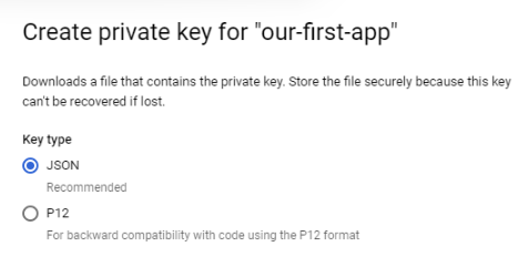
Create a Key: After creating the service account, create a key for it. Choose JSON as the key type. This key file will be used for authentication in your application.
Step 2: Add the Service Account to Google Search Console
Go to Google Search Console and sign in.
Select Your Property: Choose the website property you want to grant access to.
Navigate to Settings: Go to the settings of your Search Console property.
Manage Users and Permissions: In the "Users and permissions" section, click on "Add User."
Add Service Account Email: Enter the email address of the service account you created in Google Cloud. This email address can be found in the service account details in the Google Cloud Console.
Assign Permissions: Choose the appropriate permission level for the service account (e.g., Full, Restricted).
Step 3: Use the Service Account in Your Application
Integrate the Service Account Key: Use the JSON key file you downloaded from Google Cloud in your application to authenticate API requests.
Set Up API Client Libraries: Follow the instructions on Google Developers to set up the client library in your preferred programming language.
Make API Calls: Use the client library to make authenticated calls to the Google Search Console API.
Important notes:
So you have the service account, now what?
When you get the data from GSC, it returns in JSON format. JSON is pretty easy to use and understand across different tools and platforms. We can manipulate this data into a different, more manipulatable format, like a dataframe, or leave it as is. I’ve chosen to use a Pandas DataFrame format in this guide.
Now we have workable data, let’s work with it!
If you’re following along with the colab notebook, you can see how we use the same dataframe for all this code.
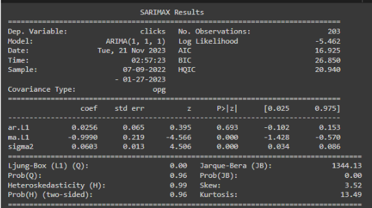
The image above shows the results you’ll get from running ARIMA. These show the variables in the code (the section under Dep. Variable), how well it fits (under No. Observations) and the parameters and residuals.
Dependent Variable (y): This is the time series data you're analyzing, which is stored in a variable, array, or list named 'y'.
Model (ARIMA(p, d, q)): This indicates the structure of the ARIMA model:
p: Number of lag observations included in the model (auto-regression).
d: Degree of differencing required to make the series stationary.
q: Size of the moving average window.
In this case, ARIMA(1, 1, 1).
Sample: Total data points in the time series.
Covariance Type: Specifies the method used to estimate the uncertainty of the model’s parameters.
No. Observations: Number of data points used in the analysis.
Goodness of Fit:
Parameters:
Residuals: the differences between the observed data and the model's predictions. Ideally, these should resemble white noise if the model fits well.
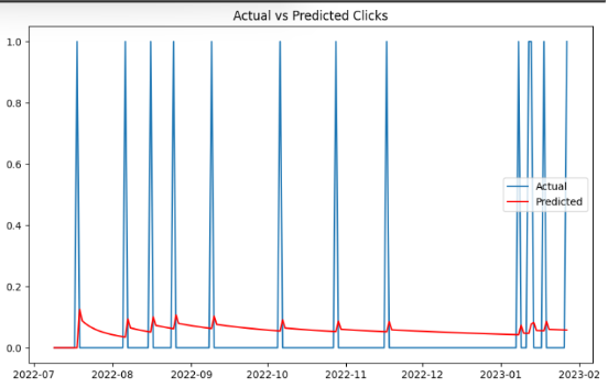
Chart showing actual number of clicks for a time period (in blue) and predicted (in red).
How to understand the results:
Model Fit: After fitting an ARIMA model to your SEO data, the first thing to look at is how well the model fits the historical data. This can be assessed using various statistical measures like the Akaike Information Criterion (AIC), Bayesian Information Criterion (BIC), and others.
Forecasting: The primary output of an ARIMA model is the forecast of future values. This forecast will give you an estimate of future trends in your SEO metrics.
Confidence Intervals: Along with the forecast, ARIMA models also provide confidence intervals, which give a range within which the future values are likely to fall. This helps in understanding the uncertainty in the predictions. I really like some of the information in statistics done wrong about confidence intervals: “A confidence interval is a range of values, derived from a set of data, that is likely to contain the value of an unknown parameter.” In plain English, it's like saying, "We are pretty sure that the true value lies somewhere within this range."
Residuals Analysis: Examining the residuals (the differences between the observed values and the values predicted by the model) is crucial. Ideally, the residuals should be random and normally distributed; any pattern in the residuals indicates that the model may not have fully captured the underlying process.
Visualization: Plotting the original data with the forecasted values and confidence intervals can provide a visual understanding of how well the model is predicting future trends.
The p-value associated with each coefficient in the SARIMA model helps you determine if the coefficient is statistically significant. In simpler terms, it tells you if a particular parameter (e.g., a specific seasonal or lag effect) is important for making accurate predictions. A small p-value (typically less than 0.05) indicates that the parameter is significant.
If you see the confidence intervals (.025 and .075) then these values represent the lower and upper bounds of the 95% confidence interval for each coefficient. In layman's terms, they give you a range within which you can be reasonably confident the true value of the coefficient falls. If the interval is narrow, it means you have a good estimate of the parameter.
When reading these results:
We can continue to use the same data with Prophet.
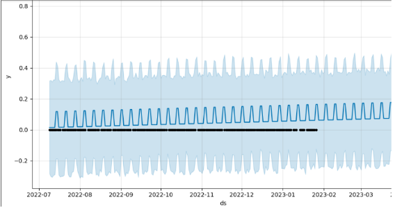
Prophet forecast and confidence interval.
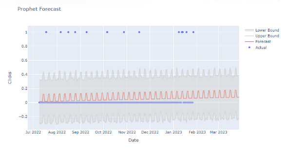
Prophet forecast vs. Actual.
Unique Prophet value propositions:
How to understand the results:
Trend Analysis: The output of Prophet includes a trend line that shows the general direction of the metric being forecasted. This helps in understanding long-term movements in SEO metrics.
Seasonality Insights: Prophet provides detailed insights into how different seasonal factors (like days of the week, months, or specific holiday periods) affect your metrics. This can be crucial for planning SEO strategies around these patterns.
Forecasting: The primary output is the forecast of future values, which includes both the expected value and uncertainty intervals.
Components: Prophet offers a breakdown of the different components (trend, seasonality, holidays) contributing to the forecast, which helps in understanding the driving factors behind the predictions.
Visualization: Visualizing the forecast along with the historical data provides a clear picture of how the forecast aligns with past trends and what future trends might look like.
Model Evaluation: Assessing the performance of the Prophet model on historical data (using cross-validation, for example) can provide insights into its accuracy and reliability.
So when reading these results:
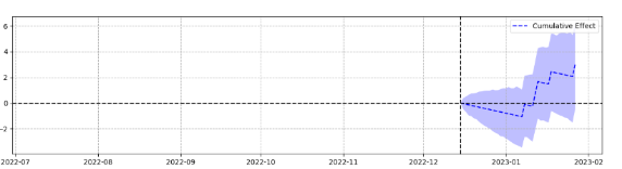
This shows an event (vertical dotted line) and the estimated impact of that event versus the predicted actual forecast, to show how big an effect the event had.

How to understand the results:
Estimated Impact: The results typically show the estimated impact of the intervention. This could be an increase or decrease in website traffic, sales, etc., due to the event.
Confidence Interval: The results will include a confidence interval for the estimated impact. This interval gives a range in which the true impact likely falls, indicating the level of uncertainty in the estimate.
Visualizations: Often, the results are accompanied by graphs showing the actual observed data and the counterfactual (what would have happened without the intervention). The difference between these lines indicates the impact.
Statistical Significance: The results will usually indicate whether the observed impact is statistically significant. This means determining whether the observed changes could be due to random fluctuations or if they are likely the result of the intervention.
Pre- and Post-Intervention Analysis: The results will often include metrics on how the data behaved before and after the intervention, helping to understand the context of the impact.
So, when you look at Causal Impact results you can:
How to use these methods to for SEO:
ARIMA
You can use ARIMA to forecast traffic or rankings based on historical data, and also to compare the forecasted data with the actual data after implementing SEO strategies to measure success.
Facebook's Prophet
Utilize Prophet for predicting traffic trends considering seasonal variations, and analyze how well your SEO strategies align with predicted trends.
Causal Impact
Apply Causal Impact to assess the effectiveness of specific SEO changes or campaigns.
Compare the actual traffic or ranking data post-intervention with the predicted data (without intervention) to quantify the impact of your SEO efforts.
In this section, we'll delve into two real-world case studies where we employed the Causal Impact analysis method to assess the impact of specific SEO changes and events.
Case Study 1: Algorithm Update Impact
One of the common challenges in SEO is dealing with the uncertainty surrounding algorithm updates. Many SEO professionals have experienced sudden changes in rankings and traffic, often attributed to algorithmic shifts. In such cases, it's essential to determine whether an algorithm update is indeed the cause of these fluctuations.
For this case study, we had a website that witnessed a noticeable drop in organic traffic shortly after a Google algorithm update and our team was eager to understand whether the update was the root cause of this decline, or if other factors were at play.
Steps Taken:
We collected historical traffic data for the website before and after the algorithm update from GSC, going back about a year (we had some stored in our BigQuery database.)
Using the Causal Impact framework, we compared the actual traffic data post-update with a counterfactual scenario. The counterfactual scenario represented what the traffic might have been without the algorithm update. So we could see that the update had a slight negative effect: if the algo update hadn’t happened, the site’s traffic would be higher.
We also examined the confidence intervals to determine the level of uncertainty in our findings.
Results:
The Causal Impact analysis revealed that the algorithm update had indeed caused a drop in organic traffic. The confidence intervals were relatively narrow, bolstering our confidence in this assessment. This information allowed us to communicate with stakeholders and form a plan.
Case Study 2: Content Publication Impact
In the second case study, we explored the effect of publishing a high-quality article on a website's organic traffic. The goal was to provide concrete evidence that the article had a positive impact on traffic, demonstrating the value of content creation efforts.
Steps Taken:
We (again) gathered historical traffic data for the website, focusing on the period leading up to and following the publication of the article.
Employing the same Causal Impact framework, we compared the actual traffic data post-article publication with a counterfactual scenario. The counterfactual represented what the traffic might have been without the article.
To make the findings more accessible, we created visualizations that displayed the observed traffic and the counterfactual. This allowed stakeholders to see the actual impact easily.
Results:
The Causal Impact analysis provided compelling evidence that the publication of the article had a positive and statistically significant impact on organic traffic. The observed traffic exceeded the counterfactual scenario consistently after the article was published.
It can be hard to prove your worth to stakeholders: but these tools can show the impact specifically an SEO can make on a digital marketing program.
Go forth and conquer, friends!
Mathematical structure of ARIMA models
Understanding Facebook Prophet: A Time Series Forecasting Algorithm
Estimating Causal Effects on Financial Time-Series with Causal Impact
We pay our authors, speakers & team to bring you helpful content like this.
We aim to always keep our content and community free and accessible.
If you've found value in WTS, please consider supporting us through our Buy Me a Coffee initiative.

